Project Final Report

Get the PDF

Chemical Reaction Simulation at Concentration and Particle Granularities with Open MP

Andrew Kubaney (ajkubane) and Haoyu Zhang (haoyuzha)

I. Summary

​ We implemented a two-dimensional chemical reaction simulator that can simulate a combination of concentration regions and particle regions in the same scene. Parallelizing this simulator with OpenMP, we were able to achieve a total speedup of 5.6 for a 200,000 particle simulation over 200 iterations on the 8-core Gates-Hillman Center (GHC) machines. The speedups and amount of cache misses for several sub-routines were examined to explain the less-than-perfect speedup. Additionally, we were able to achieve a total speedup of 22.23 for a 200,000 particle simulation over 200 iterations with 64 cores on the Pittsburgh Supercomputing Center (PSC) Bridges-2 machines. This work was complemented by the development of visualization software, allowing us to represent the iteration-by-iteration results of the simulations as a GIF.

II. Background

​ In this project, a combined concentration and particle chemical simulation was developed. The necessary chemical background to understand the simulation, an overview of the sequential algorithm, the important data structures, and the characteristics of the work are described below.

Chemical Background

​ At the scale of the atoms and molecules (collectively referred to as particles), gravitational forces are small enough to be considered negligible; however, charged particles exert significant electrostatic forces on other charged particles. Similar in form to Newton’s law of gravity, Coulomb’s law defines the electrostatic force of particle i on particle j (${\bf{F_{i,j}}}$)$^1$:

\[{\bf{F_{i,j}}} = \frac{k \cdot q_i \cdot q_j \cdot ({\bf{r_j}} - {\bf{r_i}})}{\parallel{\bf{r_j}} - {\bf{r_i}}\parallel^3}\tag{eqn. 1}\]

In equation 1 above, k is Coulomb’s constant, $q_i$ and $q_j$ are the charges of particle i and particle j, $\bf{r_i}$ and $\bf{r_j}$ are the position vectors of particle i and particle j, and $\parallel{\bf{r_j}} - {\bf{r_i}}\parallel$ is the magnitude of the vector ${\bf{r_j}} - {\bf{r_i}}$. Importantly, as with Newton’s law of gravity, Coulomb’s law is an inverse-square law, which allows the total force on a particle to be approximated by considering a subset of nearby particles. There are several important differences between Newton’s law of gravity and Coulomb’s law. First, unlike the mass of a particle, the charge of a particle can only take integer values, and the charge can be positive or negative. Second, while the gravitational force between two particles is only attractive, the electrostatic force between two particles can be attractive or repulsive. Specifically, if two particles have charges with the same sign, then the electrostatic force between the particles will be repulsive. Otherwise, if the two particles have charges with opposite signs, then the electrostatic force between the particles will be attractive.

​ Two particles collide when the sum of their radii is less than the distance between the particles. One important property of all collisions is that the total momentum (momentum is the product of a particle’s mass and its velocity vector) must be conserved (the sum of the momenta of the particles before the collision must equal the sum of the momenta after the collision). For the sake of simplicity, in this project, it was assumed that the collisions were elastic, which means that energy is conserved across the collision. Using the conservation of momentum and the conservation of energy, it is possible to derive expressions for the final velocities of two particles after a collision$^2$:

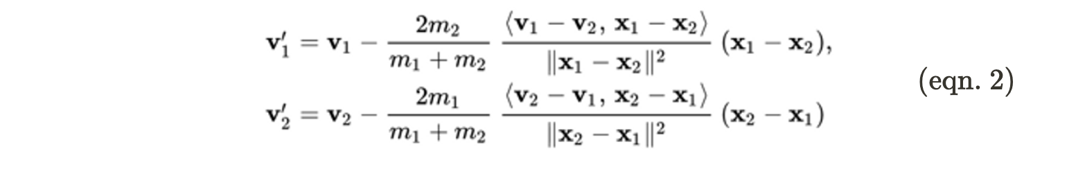
In equation 2 above, $\bf{v_1’}$ and $\bf{v_2’}$ correspond to the final velocities of the two particles, $\bf{v_1}$ and $\bf{v_2}$ correspond to the velocities of the two particles before the collision, $m_i$ and $m_j$ are the masses of the two particles, $\bf{x_1}$ and $\bf{x_2}$ are the position vectors, and $<a,b> = a \cdot b$.

​ A chemical reaction involves the transformation of particles into different particles. Chemical reactions can be reversible, which means that the transformation can happen in reverse. For the purposes of this project, we consider the following reversible chemical reaction:

​
\({A + B \leftrightarrow C}\tag{eqn. 3}\)

Note, reversible reaction from equation 3 can be represented as two reactions:

\[{A + B \rightarrow C}\tag{eqn. 4}\] \[{C \rightarrow A + B}\tag{eqn. 5}\]

The particles on the left side of the arrow are called reactants, and the particles on the right side of the arrow are called products. In the reaction depicted by equation 4 (referred to as the forward reaction), a particle of type A and a particle of type B combine to form a particle of type C. In order for this to occur, a particle of type A must collide with a particle of type B. Note, not every collision between particles of these types results in a reaction. In the real-world, this is dependent on factors such as temperature and orientation of the particles; however, for the purposes of our simulation, it is reasonable to utilize a probability. In the reaction depicted by equation 5 (referred to as the backward reaction), a particle of type C can spontaneously decompose into a particle of type A and a particle of type B. This does not happen on every time step; instead, it is also dictated by a probability.

​ In two dimensions, the concentration of a molecule of type T (denoted as $[T]$) in a region R can be calculated by dividing the number of molecules of type T in region R by the area of region R. Chemical reactions can also be simulated at a concentration level. Specifically, the rate of forward reaction from equation 4 in a concentration region R can be calculated with the following formula:

\[{Rate = k_{forward}[A][B]}\tag{eqn. 6}\]

In equation 6 above, $k_{forward}$ is the forward reaction rate constant, and $[A]$ and $[B]$ are the concentrations of type A particles and type B particles in region R. Similarly, the rate of the backwards reaction from equation 5 in a concentration region R can be calculated with the following formula: \({Rate = k_{backward}[C]}\tag{eqn. 7}\)

In equation 7 above, $k_{backward}$ is the backward reaction rate constant, and $[C]$ is the concentration of type C particles in region R. The rate is negative for the reactants of the reaction, and the rate is positive for the products (in other words, reactants are consumed, and products are formed). In order to calculate the new concentrations, the rate can be multiplied by the length of the time step to determine the change in the old concentrations.

Motivation for Combined Particle-Concentration Simulation

​ In order to understand the motivation for the combined particle-concentration simulation, it is useful to consider a possible application. Cells in the human body are many orders of magnitude larger than particles. As such, they contain far too many particles to simulate with a particle simulation. However, oftentimes, scientists may be interested in the behavior of a very small region of a cell (small enough to be simulated with a particle simulation). One solution would be for scientists to ignore the rest of the cell and only simulate the particles in the region of interest. However, due to the highly connected nature of biochemical processes in cells, this is likely to lead to inaccuracies. One solution is to simulate the large regions surrounding the region of interest at a concentration level. The concentration simulations are much time and space efficient than the particle simulation; only one value needs to be stored and updated per type of molecule per concentration region. While the concentration simulation may be less accurate than a particle simulation, it still allows for the regions outside the area of interest to have some effect on the area of interest. Thus, this chemical simulation allows for both concentration and particle regions in the same scene.

Important Data Structures and Operations

​ In our simulation, particles are represented as structs containing an identification number, a type identifier, a two-dimensional position vector, and a two-dimensional velocity vector. Since each particle of a given type has the same mass, radius, and charge, only the type is stored with the particle, and the relevant masses, radii, and charges are stored in a single vector. One important operation is the “compute force” operation. Given two particles and a culling radius, this operation uses equation 1 to compute the two-dimensional force vector that one particle exerts on the other. Another operation for particles is the update operation. Given a force vector, a time step, and the particle data, the update operation outputs a particle with the velocity and position that are a result of applying the force to the particle. Another important operation for particles is the collide operation. Given two particles that are colliding, this operation updates the velocities of the two particles according to equation 2 above. Finally, the forward reaction operation and the backward reaction operation are crucial; given that a reaction will occur, each of these operations takes the particle data corresponding to the reactants of the reaction and computes the particle data for the product of the reaction.

​ Concentration regions are also represented as structs, containing an identification number, two vectors used to represent the bounds of the region, and an array containing the concentrations of each particle type in that region. One important operation for concentration regions is the update operation. Applying equations 6 and 7 from above, this operation updates the concentrations of each particle type with the concentration region. The “generate particle” subroutine is also critical. Given a concentration region, this operation uses a pseudo-random number generator (PRNG) to generate particles of each type along the boundary of the concentration region. This is useful for allowing for interaction between concentration and particle regions. Finally, the recapture operation scans all of the particles, and for any particle that falls within the bounds of the concentration region, it deletes that particle and increases the corresponding concentration.

​ The most crucial data structure for our implementation is a quadtree. A quadtree recursively subdivides two-dimensional space into four quadrants$^3$. Each non-leaf node in the quadtree has exactly four children, and each child corresponds to one spatial quadrant. Internal nodes in a quadtree do not store particles; all particles are stored in leaves. Consider the following example of a quadtree$^3$:

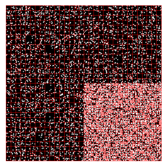
Figure 1. An example of a quadtree from the Assignment 3 writeup. The white dots represent particles, and the red lines represent the quadrants that each leaf node is assigned.

There are two important operations on quadtrees: build and “get particles.” The build operation allows for the construction of a quadtree from a vector of particles. The “get particles” operation takes in a particle and a radius and uses the quadtree to return a vector containing all particles that are within a distance of “radius” from the particle.

Overview of the Algorithm

​ There are two inputs to our algorithm: a text file and the number of iterations to run the simulation. The text file contains lists of the radii, masses, and charges for all types of particles. The text file also contains a list of all of the particles with their associated data. Finally, it contains a list of all the concentration regions and their associated data. The output of the algorithm has the exact same format as the input; however, the particle list and concentration region list now contain the particle and concentration data after the simulation was run for the given number of iterations on the input. Every iteration of the simulation contains the following steps.

1. Simulation of concentration regions.

2. Generation of particles from concentration regions

3. Simulation of electrostatic forces between particles.

4. Simulation of collisions and reactions between particles.

5. Recapturing particles into the concentration regions.

​ The sub-routine for the simulation of concentration regions is straightforward. For each concentration region, the algorithm applies equations 6 and 7 to calculate the rates of the forward and backward reaction. Then, using the length of the time step, the changes in the concentrations of each particle type are calculated and applied.

​ The next step of the generation of particles along the edges of each concentration region. This is necessary to account for the interaction between particle-simulated and concentration-simulated regions and to allow for diffusion of particles from concentration-simulated regions to particle-simulated regions. For each concentration region, the edge is defined as any area that is within a distance of the culling radius to the outside of the concentration region. This sub-routine calculates the area of this edge and utilizes this area and the particle concentrations to determine the number of particles of each type to generate. Then, the algorithm relies on a PRNG to generate particles with random positions and velocities (note, for the sake of simplicity, only the direction of the velocities are randomized; the magnitude of each velocity is set to a default value). These newly-generated particles are added to the rest of the particles. This step of the algorithm is summarized in Figure 2 below.

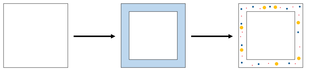
Figure 2. For each concentration region, the area of the light blue region is calculated. Then, using this area and the concentration of each particle type, as well as a PRNG, particles are generated to fill this region.

​ The simulation of electrostatic forces proceeds in a similar fashion to assignment 3. First, a quadtree of the particles is constructed. Then, for every particle i, the quadtree is queried to retrieve all other particles that are within a certain culling radius of the particle. The force of each particle within the culling radius on particle i is computed and aggregated. Then, the position and velocity of particle i are updated with the force and time step length.

​ Similar to the simulation of electrostatic forces, the simulation of collisions and reactions first requires the construction of a quadtree. For every particle i, the quadtree is queried to retrieve every particle j within the maximum particle radius across all particle types. For every particle j, this sub-routine performs a collision check. If particle i and j are colliding, and one of them is a type A particle and the other is a type B particle, then the sub-routine uses a PRNG to generate a number on the interval [0,1]. If this number is less than the specified forward reaction probability, then the particles are marked as reacted, and a particle of type C is added to a new particle vector. Otherwise, the equation 2 is used to update the momenta after the collision. After all collisions are resolved, if particle i is a type C particle, the sub-routine uses a PRNG to generate a number on the interval [0,1]. If this number is less than the specified backward reaction probability, the type C particle is marked as reacted, and a particle of type A and a particle of type B are added to the new particle vector. At the end of this sub-routine, all non-reacted particles are added to the new particle vector. There are a few features of the collision and reaction simulation that are critical for the rest of this project. First, one important trait of chemical reactions is that they conserve mass. In other words, in any given iteration, a particle should be involved in at most one reaction, and if the particle is reacted, it should be deleted. Furthermore, the collision operation is non-associative, which enforces an inherent ordering among the computation.

​ The recapturing sub-routine is relatively simple. For each particle, if it falls within the spatial bounds of any of the concentration regions, the particle is deleted. Furthermore, the corresponding concentration for that type of particle is incremented.

Workload Breakdown

​ The most computationally expensive portion of the simulation algorithm is the simulation of electrostatic forces for all particles. This amount of work necessary for this sub-routine is proportional to the density of the particles and to the culling radius. Furthermore, there are many memory accesses in traversing the quadtree. There is significant possibility for parallelism in this sub-routine. Since the calculation of each updated particle only relies on the data from the previous iteration, the per-particle update is data-parallel. Furthermore, there is spatial locality in the reading of the particle vector, and there is temporal locality in the possible re-use of nearby particles (and the associated sub trees in the quadtree). The inner loop within this simulation involves performing the same force calculation on different data, and this makes the inner loop ideal for SIMD execution. All of these factors suggest that the simulation of electrostatic forces could benefit from parallelization.

​ Another computationally expensive sub-routine is the simulation of collisions and reactions. The amount of work associated with this sub-routine is also proportional to the density of the particles; however, the amount of work is no longer proportional to the culling radius. Instead, it is proportional to the maximum particle radius, which in the simulation, was generally an order of magnitude smaller than the culling radius. Due to the conservation of mass, reactions introduce inherent dependencies (a particle can react at most once). Furthermore, the non-associativity of collisions also create dependencies in updating the collisions. There are also dependencies between all of the pseudo-random numbers; the PRNG uses the generated random number as the seed for the next random number. Unlike the electrostatic force simulation, this inner loop is not suited for SIMD execution due to the dependencies enforced by reactions and collisions. Despite these barriers to parallelization, there is a significant amount of possible temporal locality if the collisions and reactions for nearby particles are computed within a reasonable time frame. For this reason, the collision and reaction simulation could benefit from parallelization.

​ There are two sub-routines that make up a smaller fraction of the computational workload but may still benefit from parallelization: quadtree construction and the generation of particles from concentration regions. Quadtrees are built twice per iteration in this algorithm (once for the electrostatic simulation and once for the collision and reaction simulation). Due to the fact that each quadtree stores pointers to its children, there is not much locality in the construction quadtrees. Furthermore, the construction of each parent node is dependent on the construction of its children. However, the natural recursive structure of quadtree construction lends itself to a straightforward parallelization using the task-based parallelism from OpenMP, so the quadtree construction could benefit from parallelization. Similar to the collision and reaction sub-routine, the generation of particles on the boundaries of concentration regions utilizes pseudo-random numbers. As discussed before, the generation of pseudo-random numbers with a PRNG introduces dependencies between the generation of each number. Once the pseudo-random numbers are pre-generated, the construction of each particle is data-parallel. This signifies some potential for parallelization; however, the particles are only generated in the relatively small edge area of each concentration region, and this indicates that this sub-routine does not constitute a large fraction of the overall work.

​ Generally, the number of concentration regions is many orders of magnitude smaller than the number of particles. As such, simulation of concentration regions and the recapture of particles into concentration regions constitute a small fraction of the overall work. This means that parallelization of these sub-routines will not have significant impact on the total speedup for the simulation.

III. Approach

​ We relied on a combination of our solutions from Assignment 3 and Assignment 4 as the starter code for this project, and the entirety of the simulation was written in C++. OpenMP was utilized to parallelize the sequential algorithm. We designed our code with two target machines in mind: the GHC 8-core machines and the PSC Bridges-2 128-core machines. The changes made to the sequential algorithm for the purpose of parallelization, the mapping of the data structures and work across cores, and the iterations of optimization are described below.

Changes to Sequential Algorithm

​ In order to effectively parallelize the sequential algorithm, three changes were made to the sequential algorithm, and these changes are detailed below. Aside from speedup, we had two additional goals for the parallelization. The first goal was to ensure that the output of the simulation was independent of the number of processors (in other words, the output should be the same regardless of the number of processors used for the simulation). The second goal was to ensure that the output of the simulation was independent of the scheduling (in other words, running the simulation on the same input should always result in the same output). These two additional goals are difficult to implement for three reasons: the dependencies enforced by pseudo-random number generation, the non-associativity of collisions, and the inherent dependencies caused by the conservation of mass restriction. In the sections below, the changes made to the sequential algorithm are summarized.

Pre-generation of Random Numbers

​ In order to facilitate the parallelization of concentration region particle generation and the collisions and reactions of particles, all required pseudo-random numbers were pre-generated and stored in a vector. This pre-generation was completed sequentially. While the pre-generation of pseudo-random numbers alleviated the dependencies for concentration particle generation, this solution would have been inefficient for the random numbers needed for the reactions of particles. Specifically, the amount of random numbers necessary is dependent on the number of collisions. The maximum number of collisions in an iteration is $O(N^2)$ where N is the number of particles; the actual number of collisions will likely be significantly less, but this number is not easy to predict. Pre-generating $O(N^2)$ random numbers would have been computationally expensive. In order to solve this issue, we borrowed a concept from cryptography: the bitwise XOR of two independent, uniformly random numbers is also a uniformly random number$^4$. Using this concept, the necessary number of pseudo-random numbers was reduced to one for each particle (in total, N numbers). To compute a random number for each collision, the algorithm took the bitwise XOR of the pseudo-random number for each particle.

​ Other options were considered for the pre-generation of pseudo-random numbers. One consideration was to synchronize the threads’ access to the same pseudo-random number generator. However, this approach was deemed to be inefficient, and due to the dependencies of PRNG, this would have caused the output to depend on the scheduling. Another option was to allow each thread to use its own pseudo-random number generator. Again, due to the dependencies of PRNG, the output would have depended on the scheduling.

Rework of Concentration Region Particle Generation

​ The sequential version of the concentration was not conducive to parallelization across particles. In the sequential version, the outer loop was over the concentration regions, while the inner loop was over the particles that were being generated. Due to the fact that the number of particles was many orders of magnitude larger than the number of concentration regions for most scenes, it would be better to parallelize over the particles. The reordering of the loops was not trivial; the number of iterations in the inner loop (the number of particles to be generated) depended on the concentration region from the outer loop. The solution for this issue was to compute the number of each type of particle that needed to be spawned. Using these numbers to determine the concentration region and type for a particle, the algorithm looped over the particles to be generated.

Partitioning of Particles for Collisions and Reactions

​ Recall, the collision operation is non-associative, and the reaction operation has inherent dependencies due to the fact that a particle can only react once. During the simulation of collisions and reactions, each particle can affect a local neighborhood of particles (in this case, the neighborhood of a particle is defined to be all of the particles that are currently colliding with it). To eliminate the dependency of this sub-routine on scheduling, it was necessary to ensure that the total neighborhood for each processor (the union of the neighborhoods of all the particles assigned to that processor) was disjoint from the total neighborhoods of all other processors. The partitioning scheme is described in Figure 3 below.

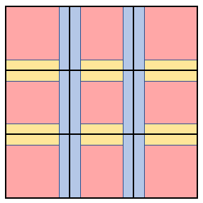
Figure 3. A 3x3 example of the partitioning scheme for the collisions and reactions sub-routine.

In the above partitioning scheme, the red blocks are referred to as the “grid partition”, the blue lines are referred to as the “vertical partition”, and the yellow lines are referred to as the “horizontal partition.” The grid, vertical, and horizontal partitions are constructed such that any two blocks within any one of these partitions are a distance of two times the maximum particle radius. As long as each processor works on a separate block, the total neighborhood of one processor will always disjoint from the rest of the total neighborhoods. The actual partitioning utilized a 12 by 12 grid. To ensure that the output of the algorithm was not dependent on the number of processors, the same grid partition was used regardless of the number of processors available (note, 12 by 12 was chosen specifically to accommodate the maximum processor count, 128). Once the particles were partitioned sequentially, the grid blocks were updated first, followed by vertical blocks, and then the by the horizontal blocks.

Mapping and Scheduling of Work

​ All of the data structures, including the quadtrees and particle vectors, were placed into shared memory. In this project, the work was scheduled using OpenMP constructs. Our implementation did not handle the explicit mapping of the work to CPU cores; instead, the mapping was handled by OpenMP.

​ The parallelization strategy for the simulation of electrostatic forces and the quadtree construction was similar to the parallelization from Assignment 3. For the electrostatic force simulation, OpenMP’s dynamic scheduling with a chunk size of 128 was used to parallelize across particles. Dynamic scheduling was chosen instead of static scheduling due to the fact that work for each particle could differ significantly (based on the local particle density). For the inner loop (the aggregation of the force calculation of nearby particles), SIMD execution was used. The quadtree construction was parallelized via OpenMP task parallelism. Specifically, for the construction of each child node, a task was spawned. Importantly, there was a cutoff of 128 particles for the spawning of new tasks; if the number of particles in a child’s quadrant was less than the cutoff, a new task was not spawned.

​ The parallelization of the concentration region particle generation was straightforward: static scheduling for loop that calculated the number of particles for each type and region, and static scheduling was used for the loop that generated the particles. Static scheduling was used in this case due to the fact that each iteration of these loops performed the exact same computation.

​ The partitioning described in Figure 3 allowed for the parallelization of the collision and reaction updates. Dynamic scheduling with a chunk size of 1 was used to parallelize over the grid partition blocks (note, the parallelization was not over particles, but rather, over spatial blocks of particles). After the grid partition blocks updates completed, dynamic scheduling with a chunk size of 1 was used to parallelize over the vertical blocks. Finally, dynamic scheduling with a chunk size of 1 was used to parallelize over the horizontal blocks. Note, dynamic scheduling was utilized because the collision and reaction runtime in each of these blocks was dependent on the density of collisions in each block, which was likely to vary across the scenes.

Iterations of Optimization

​ There were several iterations of optimization that were completed before arriving at the final parallelized algorithm. We attempted to parallelize the generation of pseudo-random numbers. In order to achieve an output that was independent of scheduling and number of processors, it was necessary to use 128 different pseudo-random number generators, each with their own seeds. With careful scheduling, the pseudo-random number generation for any amount of numbers could be parallelized across multiple cores. While this was implemented, for the scenes that were analyzed, this parallelization decreased the overall performance. We hypothesized that the overhead of scheduling the work (even with static scheduling) dominated the computation, which limited the effectiveness of the parallelization. Similar to the parallelization of random number generation, we experimentally observed that the parallelization of several other simple loops reduced the performance of the simulation. Thus, none of these parallelization strategies were included in the final version.

​ Finally, we considered multiple partitioning schemes for the collision and reaction simulation before settling on the grid-based partition. While grid-based spatial partitions are useful for limiting communication across partition blocks, this was not the driving factor of our decision. In fact, after the partitioning, there is no communication between processors during the collision and reaction updates. Instead, the grid-based partition was chosen for its ability to maximize the number of partition blocks. Given that communication was not a concern, a partition consisting of horizontal blocks would have been conceptually simpler to implement. Using this partition scheme to create 128 blocks (the maximum number of cores used in this project), the height of each horizontal block would be similar to the maximum particle radius. Recall, the partitioning only alleviates scheduling dependency if each block is separated by at least two times the maximum particle radius. Thus, with this partitioning scheme, the number of blocks would need to be reduced. This would decrease the potential for load balancing when run with a small number of processors and would leave processors idle when run with a large number of processors. Taking into account this constraint on the minimum block size, the grid-based partitioning scheme allows for a greater number of blocks (due to the fact that the space is partitioned in two dimensions as opposed to one).

IV. Results

​ The correctness of the sequential and parallel algorithms was verified, and the performances of the parallelized version on the 8-core GHC machines and on the 128-core PSC Bridges-2 machines were determined. The results for correctness and performance are discussed in the sections below. In the sections below, we refer to scenes by the number of particles that they contain. Importantly, at any given time, there may be less particles than the listed number. This is because the particle count refers to the total number of particles before any of the particles in the concentration regions are deleted.

Correctness of Sequential and Parallel Simulations

​ Verifying the correctness of the sequential and parallel simulations was not straightforward. This was due to the fact that we were not parallelizing an existing algorithm; instead, we developed our own algorithm. As such, the best way to verify correctness was to ensure that both simulations follow the high-level chemistry concepts described in the background section. Two scenes were used to evaluate the correctness of the simulations: the random_100 scene and the donut_20k scene, and these scenes are displayed in Figure 4 below.

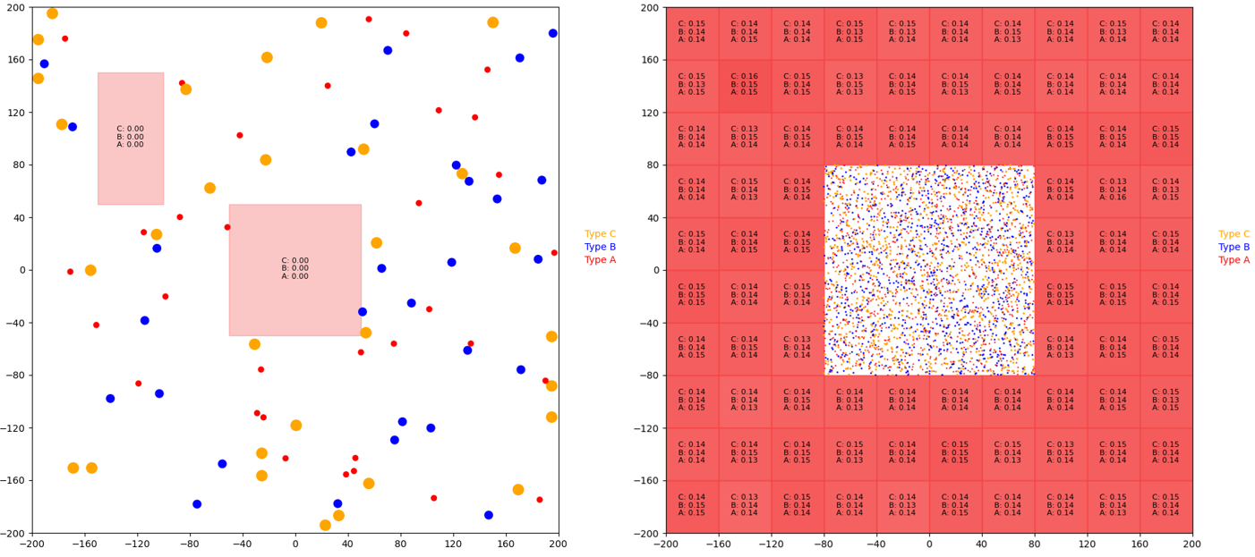
Figure 4. The random_100 scene (left) includes 100 particles and two concentration regions, and the donut_20k scene (right) contains 20,000 particles and 84 concentration regions. Type A, type B, and type C particles are red, blue, and yellow respectively. The red rectangles correspond to concentration regions, and darker rectangles correspond to more concentrated regions.

​ Each of these scenes served a different purpose for confirming correctness. The random_100 scene was simulated for 300 iterations. This scene indicated that the collisions and reactions were working correctly: many particles were observed to collide and bounce off each other, the forward reaction was observed to occur, and the backwards decomposition reaction was also observed. This scene also demonstrated the generation and capture of particles by the concentration regions. Occasionally, some particle collisions would result in the particles sticking together. This was not a bug with the algorithm; the sticking was a result of the physical parameters of the simulation. Chemical simulations are often very sensitive to the physical parameters used in the model. Finer tuned physical constants would mitigate this issue; however, for the purposes of our project, this finer tuning was not important, as it would not affect the parallelization of the workload.

​ The donut_20k scene (also simulated for 300 iterations) demonstrated that particles were diffusing from the concentration regions to the particle regions and vice versa. Additionally, the simulation of this scene revealed that the concentrations (denoted by the black text in each concentration region) for each molecule type were being updated correctly. While it is difficult to display the correctness of our simulation with images, we direct the reader to visit our online appendix. Figures A1, A2, A3, and A4 in the online appendix display GIFs of the 300 iteration simulations of these scenes for the sequential and parallel implementations.

​ Recall, one of our objectives was to make the output independent of scheduling and the number of cores. Empirical evidence suggested that this objective was achieved. Specifically, with the same input, the output of the parallelized version was recorded to be the same across multiple runs. This indicated that parallelized version was stable relative to the scheduling. With the same input, the output of the final parallelized version was recorded to be the same across multiple runs where different cores were specified. This provided evidence for the stability of the simulation relative to the number of cores.

Performance of Parallelized Algorithm on GHC Machines

​ We developed five different scenes to test the performance of the parallelized algorithm, and these scenes are displayed in Figure 5 below.

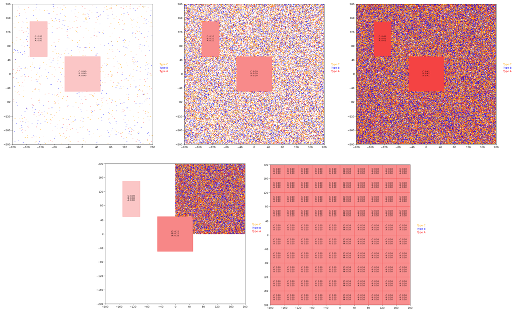
Figure 5. From left to right, (top) random_1k, random_50k, and random_200k, (bottom) corner_50k, grid. These scenes were simulated for 200 iterations to test the performance of the algorithm.

​ The problem size can scale in multiple ways, including the number of particles, the density of particles, and the total boundary area of concentration regions (the sum of the areas of the edges of the concentration regions). The scenes from figure 5 were designed to probe the different ways that the problem size can scale. The random_1k scene contains 1,000 particles and two concentration regions. The random_50k and random_200k contain the exact same concentration regions but with 50,000 and 200,000 particles respectively. These scenes were included to test the performance of the algorithm as the number of particles scales. The corner_50k scene, which has the same concentration regions as the previous scenes with all 50,000 particles pushed to the top right corner, was designed to test how the performance scales with particle density. Finally, the grid scene, which contains 100 concentration regions, was created to observe the performance as the total boundary area of the concentration regions scales. In order to determine the performance of the parallelized version, each of these scenes was simulated for 200 iterations. The total execution time, the execution times, and the speedup graphs were generated with our custom checker.py script.

​ The performance of the parallelized algorithm was quantified via speedup, and the total speedup of the parallelized algorithm was measured on the 8-core GHC machines for each of these scenes. Due to the fact that the parallelized algorithm was modified from the sequential algorithm, the total speedup was calculated as the total execution time of the parallelized simulation on N processors divided by total execution time of the parallelized simulation on 1 processor. The total speedups with 1, 2, 4, and 8 processors for each scene are displayed in Figure 6 below.

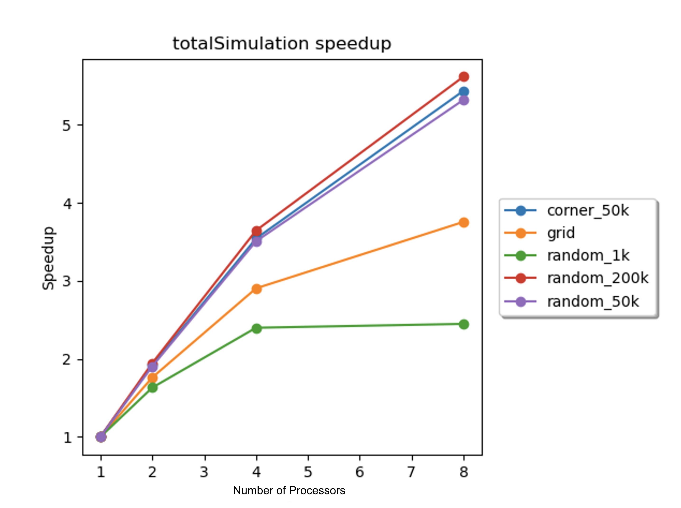
Figure 6: Total speedup vs. number of processors for each scene. Speedups were computed for 1, 2, 4, and 8 processors on the 8-core GHC machines.

While the total speedup graph demonstrates that perfect speedup was not achieved, it does not provide enough data to elucidate the cause of the less-than-perfect speedup. One piece of data that hinted at one of the potential inefficiencies was the cache miss rate. Figure 7 depicts the scaling of the cache miss rate (as a percentage) with the number of processors for each scene. To calculate the cache miss rates, the perf tool was used to measure the total number of cache references and cache misses (the cache miss rate as a percentage was the ratio of cache misses to references, divided by 100).

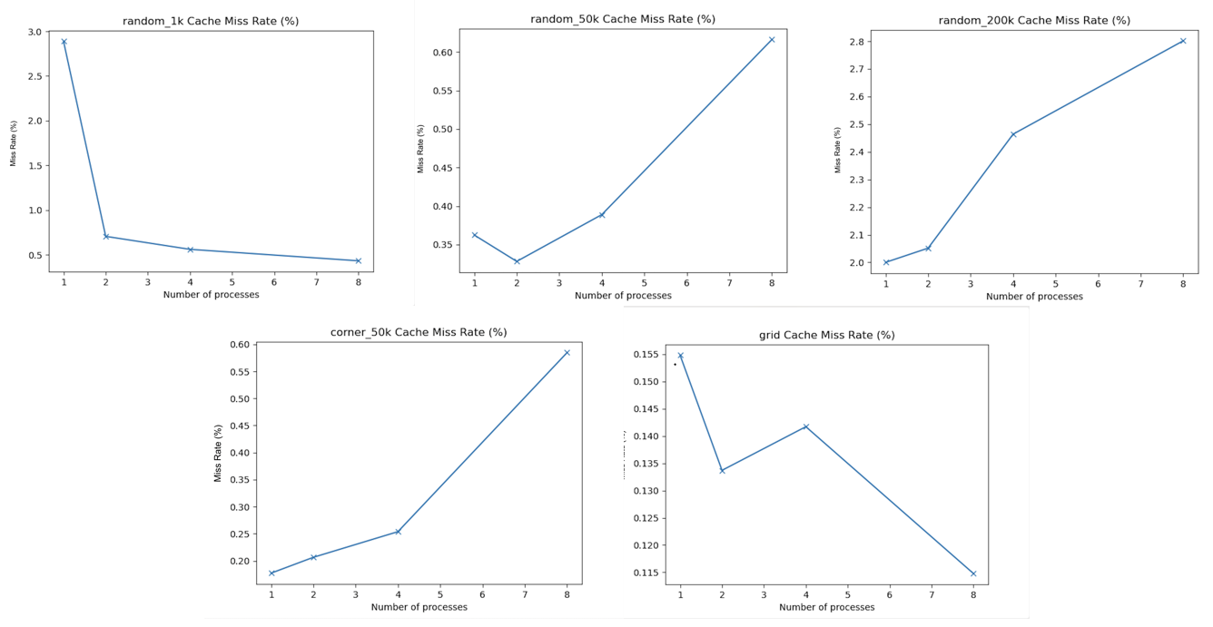
Figure 7. The cache miss rate vs. number of processor graphs, computed on the 8-core GHC machines (for 1, 2, 4, and 8 processors) for the following scenes (from left to right): (top) random_1k, random_50k, random_200k, (bottom) corner_50k, and grid.

The graphs from Figure 7 show that the cache miss rate increased with the number of processors for some of the scenes. This indicated that some of the cache misses were communication cache misses, caused by multiple processors accessing and writing to the same data structures in shared memory. It is possible these communication cache misses contributed to the imperfect speedup; however, the cache miss rate for some of the scenes decreased as the number of processors increased. To further understand the imperfect speedups, it was necessary to consider the speedups of several of the sub-routines.

​ First, the speedups for the quadtree construction and electrostatic force simulation on the 8-core GHC machines were determined with 1, 2, 4, and 8 processors for each scene. Similar to the total speedup, these sub-routine speedups were calculated as the ratio of the execution time of the parallelized subroutine on N processors to the execution time of the parallelized subroutine on 1 processor. The speedups are plotted against the number of processors in Figure 8 below.

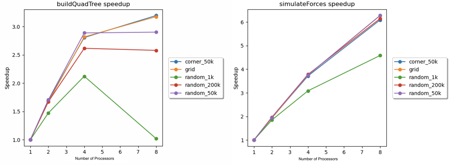
Figure 8. Speedup vs. number of processors for the quadtree construction (left) and the electrostatic force simulation (right) on the 8-core GHC machines for each scene.

​ The above speedup graphs demonstrate that the speedups for the construction of the quadtree were significantly less-than-perfect. We hypothesize that the imperfect speedup was caused by a combination of stalls due to cache misses and synchronization stalls. The data from Table 1 below supports the hypothesis related to cache misses. Table 1 shows that a significant percentage of the overall cache misses occurred in the buildQuadTree function. These cache misses were likely due to the structure of the quadtree: the children were stored as pointers. Since the quadtree was not stored in contiguous memory, there was a significant lack of spatial locality. While we have no timing data to support the presence of synchronization stalls, we believe that the sub-routine’s use of the “pragma omp taskwait” in the construction of every parent node created ample opportunities for synchronization stalls.

​ The speedups for the simulation of electrostatic forces were also imperfect. From Figure 8, it can be deduced that load balancing was not the issue here. As the corner_50k progressed, the particles diffused away from the high-density corner, leading to disparate densities across the scene. Despite this, the speedup for the corner_50k scene was similar to the speedups for the random_50k and random_200k scenes. This indicated that the dynamic scheduling utilized in the simulation of electrostatic forces was effective at balancing the workload. While the random_50k and random_200k scenes displayed similar speedups for both subroutines, the speedup for the random_1k scene was significantly lower. We hypothesize that this was due to the relatively low number of particles. Specifically, this would be an issue for two reasons. First, task-based parallelism and dynamic scheduling in OpenMP both have implicit overhead and synchronization costs. If the number of particles is too small, the efficiency gains from parallelizing the work are offset by the implicit overhead and synchronization costs. Second, in order for the load balancing to be effective, the number of tasks must outnumber the number of processors. However, since the dynamic scheduling had a chunk size of 128, the 1000 particles were decomposed into 8 chunks, which was likely not enough to ensure good load balancing.

​ In order to explain the imperfect speedups for the rest of the scenes, the data from Table 1 are useful. While the percentage of total cache misses ascribed to the simulateForces function was relatively low for all scenes, the percentage of cache misses for the getParticlesImpl function were non-negligible. The simulateForces function uses the getParticlesImpl to query the quadtree to get all of the particles within the culling radius of a particle. Traversing a quadtree involves pointer traversal between every parent-child pair. This leads to poor spatial locality, which explains the large number of cache misses.

/project-campfire-website/assets/images/2022-12-18

Table 1: Percentage of Total Cache Misses for Important Sub-routines and Scenes.

​ Table 1 includes the percentage of total cache misses attributed to various sub-routines for each of the scenes. The values in the table were generated via perf report and perf record, by running the simulation with 8 cores on the GHC machines. Note, for the scene_random_1k, we increased the sampling rate using the tag “-c 10” in order to observe enough cache misses. One interesting finding is that for scenes involving intensive particle computations, i.e., random_200k, random_50k and corner_50k, function call _M_realloc_insert() contributes a majority of cache misses. This is because we relied on vector.push_back()$^5$,which essentially calls the previous function, extensively to store newly generated particles from all kinds of sources. A C++ vector will resize its capacity once it’s full. Resizing is usually not in-place, meaning a new vector with a larger capacity with some other memory address will be created, and all the old data is read and written to the new vector. This will lead to a considerable amount of capacity misses when the working set is huge (which is true for the three scenes). This suggests a potential improvement for both our parallel and sequential algorithms: reduce the reliance on vectors for storage. While vectors were a convenient container, this demonstrated that there was a computational price for this convenience.

​ The speedups for the concentration region particle generation sub-routine on the 8-core GHC machines were determined with 1, 2, 4, and 8 processors for each scene, and a plot of the speedups against the number of processors is displayed in Figure 9 below.

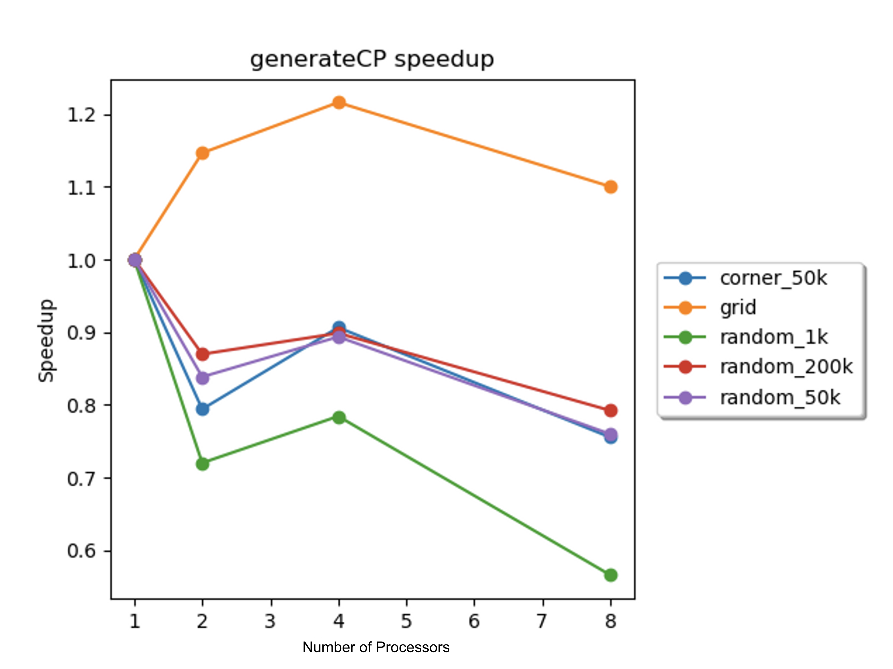
Figure 9. Speedup vs. number of processors for the concentration region particle generation sub-routine on the 8-core GHC machines for each scene.

The most disappointing speedup results were found in the concentration region particle generation sub-routine. For most of the scenes, the speedup was less than 1, which indicated that the parallelization hurt performance. For the grid scene, the speedup was slightly above one. This agreed with our expectation for this scene: the performance was better for a scene with a larger total concentration region boundary area. This slight scaling of the performance for the grid scene indicated the issue with the parallelization for the rest of the scenes: the amount of particles generated for each iteration was relatively low compared to the total number of particles. For the random_50k scene, the number of concentration region particles generated per iteration, which was around 1,000, was significantly less than the total number of particles in the scene. Due to the low number of generated particles, the poor performance was likely caused by the same issues that caused the previously-explained poor performance for the random_1k scene. Recall, in order to parallelize the algorithm, the loops for this sub-routine were reordered. The overhead from this reordering, along with the inherent overhead from OpenMP scheduling, outweighed the benefit gained from parallelization. Another possible contributing factor was cache misses. Reordering the loops involved necessitated the usage of vectors to store important intermediate numbers. While the percentage of cache miss for concentration region particle generation (generateCP) were low, compared to the relatively small amount of particles that were generated per iteration, these cache misses potentially contributed to the imperfect speedup.

​ The speedups for the simulation of collisions and reactions on the 8-core GHC machines were determined with 1, 2, 4, and 8 processors for each scene, and a plot of the speedups against the number of processors is displayed in Figure 10 below.

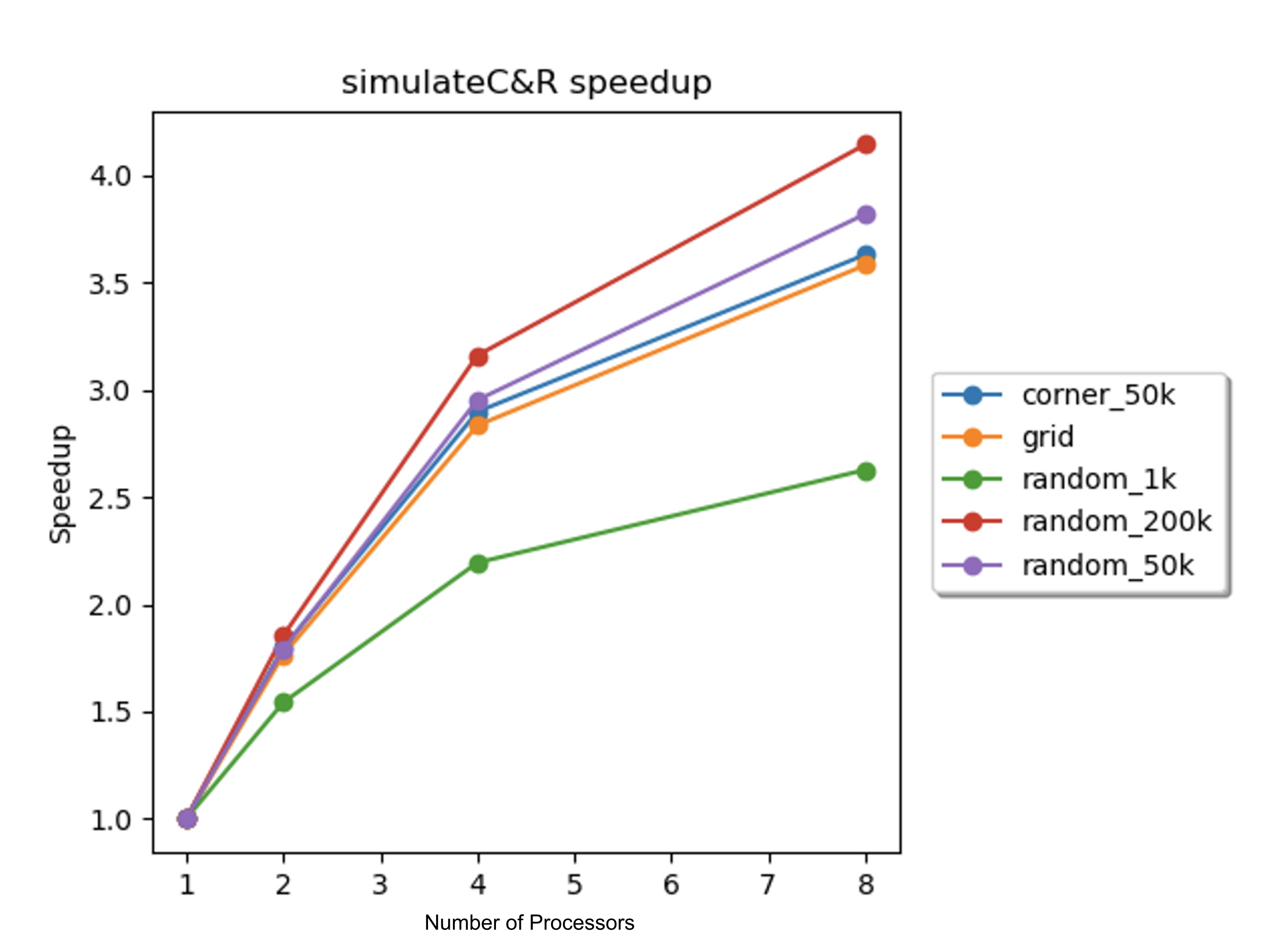
Figure 10. Speedup vs. number of processors for collision and reaction simulation on 8-core GHC machines for each scene.

As displayed in Figure 10 above, the speedups for the collision and reaction simulation across all scenes were imperfect. As with the simulation of electrostatic forces, the speedup for the corner_50k scene was similar to the speedups for the random_50k and random_200k scenes. This indicated that the dynamic scheduling of blocks was sufficient to achieve good load balancing, and as such, the imperfect speedup was not likely to be caused by load balancing issues. For the random_1k scene, the explanation for the poor speedup is similar to the explanation presented in the discussion of the simulation of electrostatic forces: the small amount of work makes good load balancing unlikely and the benefit from parallelizing a small amount of work is outweighed by the implicit overhead and synchronization costs of the OpenMP dynamic scheduling.

​ According to Table 1, the total percent of cache misses corresponding to the collision and reaction simulation was significant for the particle-heavy scenes. Recall, near the beginning of this analysis, from Figure 7, it was determined that communication cache misses were present in the algorithm. At least some of the cache misses associated with this sub-routine were likely communication cache misses. While this sub-routine had high temporal locality due to the spatial decomposition of particles, the spatial decomposition also resulted in low spatial locality. This was due to the fact that the particles appeared randomly in the particle vector (they were not grouped by position). Thus, the spatial partitioning (as opposed to the chunked partitioning of the particle vector from the electrostatic force simulation) resulted in effectively random accesses to the particle vector and another vector used for tracking reactions. With multiple processors making random accesses into these vectors, false sharing was likely to occur, which would explain the communication cache misses. Finally, in the Approach section above, we described that the partitioning for this sub-routine was done sequentially. According to Amdahl’s law, due to the fact that this non-negligible part of the algorithm was sequential, the speedup for the collision and reaction simulation was limited.

​ In order to determine where there is room for improvement, it is useful to consider the percentage of the total execution time associated with the four sub-routines described above (construction of the quadtree, simulation of electrostatic forces, generation of concentration particles, and simulation of collisions and reactions). These percentages, computed with 1, 2, 4, and 8 processors on the GHC machines, for the random_200k and grid scene are displayed in Table 2 below.

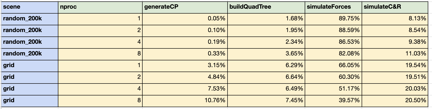
Table 2: Percentage of Total Execution Time for each Sub-routine

Table 2 suggests that the most dominant computation is the simulation of electrostatic forces; however, this sub-routine also had the best speedup. Although the other sub-routines made up smaller percentages of the overall execution time, we would argue that they are more ripe for improvement. First, the speedups for these sub-routines were significantly worse than the speedup for the simulation of electrostatic forces. Second, many chemical reactions occur between neutrally charged particles (particles with a charge of 0). There would be no electrostatic forces to simulate, so the entire sub-routine could be removed. In this case, the other three sub-routines would constitute a much greater percentage of the overall execution time.

​ Given the above performance analyses and the characteristics of the simulation, we believe that our choice of machine target (CPU) was sound (over the alternative of a GPU). While the simulation of electrostatic forces was readily data parallel, the rest of the sub-routines had significant dependencies. This would make the parallelization of these sub-routines with a GPU difficult. Furthermore, the simulation of electrostatic forces and the simulation of collisions and reactions make a large number of memory accesses. As such, the arithmetic intensity might be too low to justify parallelization on a GPU.

Performance of Parallelized Algorithm on PSC Machines

​ The parallelized algorithm was used to simulate the five scenes from the previous section for 200 iterations on the 128-core PSC Bridges-2 machines. These simulations were conducted with 1, 2, 4, 8, 16, 32, 64, and 128 processors, and the speedups were calculated in the same way as the previous section. These speedups are plotted versus the number of processors in Figure 11 below.

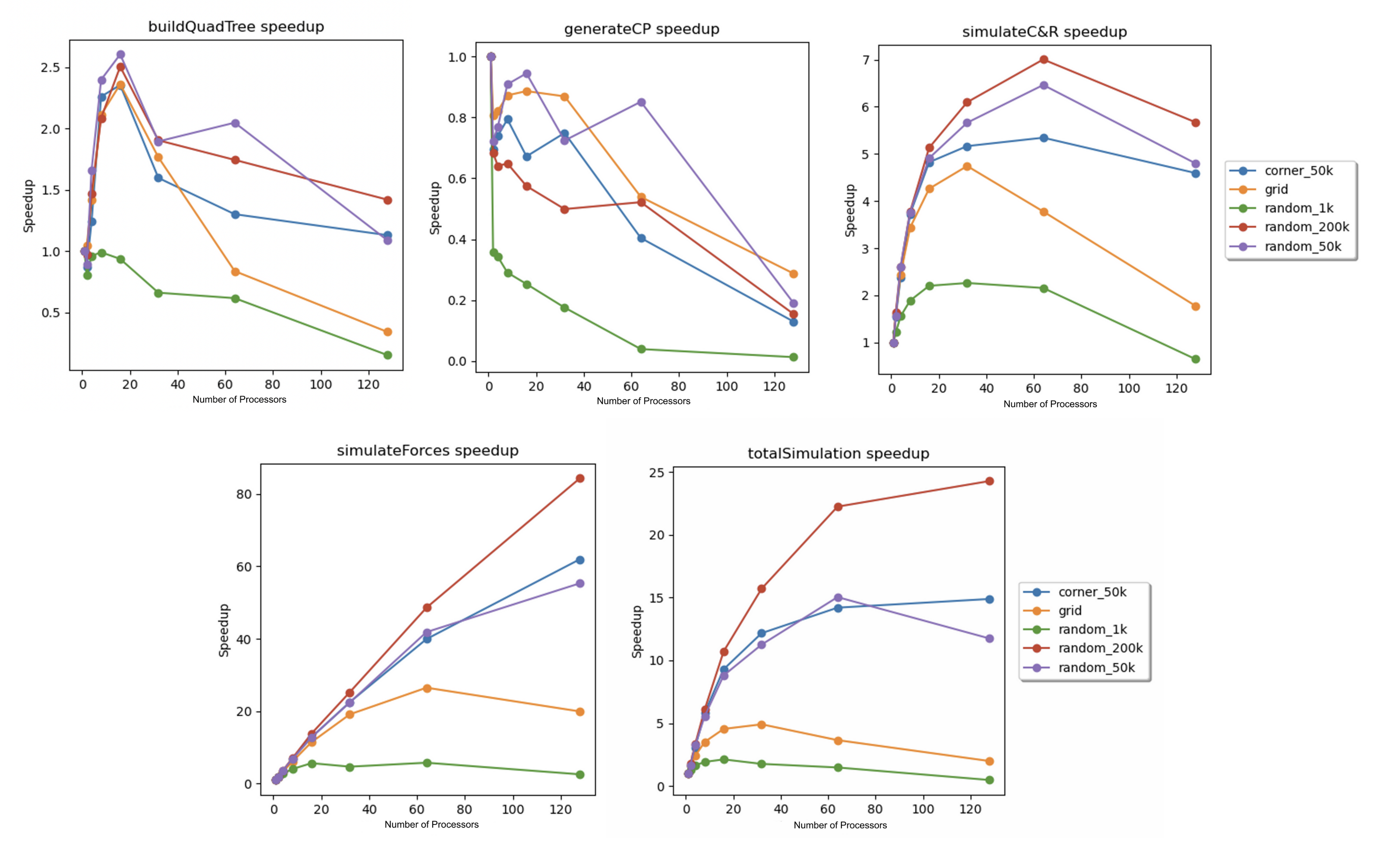
Figure 11. Speedup vs. number of processors for (from left to right): (top) quadtree construction, concentration region particle generation, simulation of collisions and reactions, (bottom) simulation of electrostatic forces, and the total simulation for every scene.

​ Due to time constraints, a more in-depth analysis of the parallelized simulator on the PSC machines was not possible. From the above speedup graphs, the total speedups and the speedups for each sub-routine were significantly less-than-perfect. Many of the trends explained in the above section were extended in these speedup graphs. The most significant unexplained trend was the noticeable drop in speedup for the collision and reaction simulation as the number of processors increased from 64 to 128. One possible explanation involves the fact that the number of blocks in the grid partition was static (it was always a 12 by 12 grid, so there were 144 grid blocks regardless of the number of processors). As the number of processors increased from 64 to 128, many of the processors only received one grid block. This severely limited reduced the capability of the dynamic scheduling to produce a good load balance, which may have contributed to the decrease in performance.

V. Future Directions

​ While we completed our goals and deliverables, as we completed the project, we noticed several directions that would be interesting to explore in the future. First, we recognize that the shared address space model of OpenMP limits the ability of our code to scale for supercomputers that contain large clusters of machines. Since chemical simulations are often run on these types of supercomputers, it would be useful to implement a parallel version using a message passing interface (such as OpenMPI), which would scale better.

​ As displayed above, the parallelization of the concentration region particle generation resulted in speedups that were less than one for most of the scenes. While this may indicate that this parallelization should be removed, a more nuanced improvement would involve setting cutoffs for the number of particles to be generated (if the number of particles to be generated was less than the cutoff, a sequential algorithm would be used instead).

​ According to the above analyses, the most logical next step for optimization would be the parallelization of particle partitioning. As discussed above, the fact that the particles were sequentially partitioned in the parallelized algorithm limited the overall speedup. As such, parallelizing this part of the code would present the greatest opportunity to improve the performance of the simulation.

​ Another interesting direction would be the creation of more complicated input scenes. Since this simulation allows for concentration and particle regions in the same scene, the number of interesting scenes is much larger than the number of interesting scenes for particle-only simulations. Developing more complicated scenes would push the limit of the parallelization. Finally, it would be instructive to attempt to match our chemical simulation to real-world chemical reactions. This would involve researching experimental details of these chemical reactions and translating these details into the physical constants used by the simulation. If the simulation’s output matched the experimentally determined results, this would further support our confidence in the correctness of our simulation.

References

$^1$Coulomb’s Law. http://hyperphysics.phy-astr.gsu.edu/hbase/electric/elefor.html.

$^2$Elastic Collision. https://en.wikipedia.org/wiki/Elastic_collision.

$^3$15-418 Course Staff. Assignment 3 Writeup, https://www.cs.cmu.edu/afs/cs/academic/class/15418-f22/public/asst/asst3/asst3.pdf.

$^4$Patarin, Jacques. A Proof of Security in O(2n) for the Xor of Two Random Permutations, Information Theoretic Security, Third International Conference, ICITS 2008, Proceedings, p. 232, https://link.springer.com/book/10.1007/978-3-540-85093-9.

$^5$Kushashwa Ravi Shrimali. Understanding how Vectors work in C++ (Part-1): How does push_back work?, https://krshrimali.github.io/posts/2020/04/understanding-how-vectors-work-in-c-part-1-how-does-push_back-work/.

Breakdown of Work and Total Credit

Work

• Andrew Kubaney
  • Wrote sequential chemical simulator
  • Completed simple parallelization of chemical simulator with OpenMP.
  • Parallelized collision and reaction algorithm and concentration region particle generation algorithm.
  • Analyzed results.
• Haoyu Zhang
  • Wrote visualization software.
  • Wrote code to analyze sequential and parallel simulator.
  • Generated speedup and cache miss graphs.
  • Analyzed results.

Total Credit

• Andrew Kubaney: 50%
• Haoyu Zhang: 50%